Periodic functions. Periodicity of trigonometric functions. ☰

Periodic functions are functions that repeat their values in regular intervals or periods. The concept of periodicity is important in various branches of mathematics, such as Fourier analysis and signal processing. A function \(f(x)\) is said to be periodic if there exists a non-zero constant P such that for all \(x\) in the domain of \(f\), the following condition holds:
\(f(x+P)=f(x)\).

The smallest positive value of \(P\) for which this condition is satisfied is called the period of the function.

Trigonometric functions, such as sine and cosine, are fundamental examples of periodic functions. Let's discuss the periodicity of the sine and cosine functions:

Sine function: The sine function, denoted by \( sin(x) \), is periodic with a period of \( 2 \pi \). This means that for all \(x\):
\( sin(x+2 \pi )=sin(x) \).

In other words, the sine function repeats its values every \( 2 \pi \) units along the \(x\)-axis.

Cosine function: The cosine function, denoted by \(cos(x) \), is also periodic with a period of \( 2 \pi \). This means that for all \(x\):
\( cos(x+ 2 \pi )=cos(x) \).

Like the sine function, the cosine function also repeats its values every \( 2 \pi \) units along the \(x\)-axis.

The tangent function, denoted by \( tan(x) \), is another example of a periodic trigonometric function. However, its period is different from sine and cosine functions. The tangent function has a period of \( \pi \), which means that for all \(x\):
\( tan(x+ \pi )=tan(x) \).

The tangent function repeats its values every \( \pi\) units along the \(x\)-axis.

In summary, trigonometric functions are periodic functions, with the sine and cosine functions having a period of \( 2 \pi \), and the tangent function having a period of \( \pi \). These periodic properties are essential in solving trigonometric equations and analyzing periodic phenomena in various scientific and engineering applications.

Graphs of the functions sine (y=sin(x)) and cosine (y=cos(x)) ☰

The graphs of the sine and cosine functions, \( y=sin(x) \) and \(y=cos(x) \), are essential for understanding their properties and behavior. Both functions are periodic and oscillate between \(-1\) and \(1\). The graphs exhibit the periodicity and amplitude of these functions. Let's discuss the graphs of both functions in detail.

Graph of \( y=sin(x) \) :
The sine function has a period of \( 2 \pi \). This means that it repeats its values every \( 2 \pi \) units along the \(x\)-axis. The graph of the sine function starts at the origin \((0,0)\) and oscillates between \(-1\) and \(1\) with some key points:
\( x = \frac{ \pi }{2} \), \( sin(x)=1 \) (maximum value)
\( x = \pi \), \( sin(x) = 0 \) (zero crossing)
\( x= \frac{3 \pi }{2} \), \( sin(x)= -1 \) (minimum value)
\(x=2 \pi \), \( sin(x)=0 \) (zero crossing and one complete cycle)

The sine function has a wave-like shape, and its graph is symmetric with respect to the origin (odd function). The graph extends infinitely in both the positive and negative \(x\) directions, repeating its pattern every \(2 \pi \) units.


Graph of \(y=cos(x) \):
The cosine function, like the sine function, has a period of \(2 \pi \) and oscillates between \(-1\) and \(1\). However, the graph of the cosine function is phase-shifted by \( \frac{\pi}{2} \) units to the left compared to the sine function. Here are some key points for the cosine function:
\( x =0 \), \( cos(x)=1 \) (maximum value)
\( x = \frac{ \pi }{2} \), \( cos(x)=0 \) (zero crossing)
\( x = \pi \), \( cos(x)= -1 \) (minimum value)
\( x= \frac{3 \pi }{2} \), \( cos(x)=0 \) (sıfır nöqtəsi)
\(x = 2 \pi \), \( cos(x)= 1\) (zero crossing and one complete cycle)

The cosine function also has a wave-like shape, and its graph is symmetric with respect to the \(y\)-axis (even function). The graph extends infinitely in both the positive and negative \(x\) directions, repeating its pattern every \( 2 \pi \) units.

In summary, the graphs of the sine and cosine functions are periodic wave-like patterns that oscillate between \(-1\) and \(1\). They have a period of \( 2 \pi \), with the cosine function being phase-shifted by \( \frac{\pi }{2} \) units to the left compared to the sine function. These graphs help to visualize the properties and behavior of the sine and cosine functions, which are fundamental in trigonometry and various applications in mathematics, science, and engineering.

Transformations of sine and cosine functions☰

Transformations of sine and cosine functions involve modifying the basic sine and cosine functions to create new functions with different properties, such as amplitude, period, phase shift, and vertical shift. These transformations allow us to model a wide range of periodic phenomena in various fields, such as physics, engineering, and music. The basic sine and cosine functions are given by:
\( f(x) = sin(x) \)
\( g(x) = cos(x) \)

Here's a brief overview of the four common transformations:

Amplitude: The amplitude is the peak value of the function, or the maximum distance from the function's central axis. Changing the amplitude involves multiplying the sine or cosine function by a constant, denoted by "\(A\)":
\( f(x)= Asin(x) \)
\( g(x) = Acos(x) \)

If \( A > 1 \), the amplitude increases, and if \( 0 < A < 1 \) , the amplitude decreases. If \(A\) is negative, the function is reflected over the horizontal axis.

Period: The period is the interval over which the function repeats itself. To change the period of the sine or cosine function, we multiply the input variable \((x)\) by a constant, denoted by "\(B\)":
\( f(x) = sin(Bx) \)
\( g(x) = cos(Bx) \)

The new period of the function is found by dividing the original period (\( 2 \pi \) for both sine and cosine functions) by the absolute value of \(B\):
\( \text{New period } = \frac{2 \pi }{ |B| } \). If \( B > 1 \) , the function is compressed horizontally, and if \( 0 < B < 1 \) , the function is stretched horizontally.

Phase Shift: The phase shift is a horizontal shift of the function. It's achieved by adding or subtracting a constant, denoted by "\(C\)", from the input variable \((x)\):
\( f(x) = sin( B \cdot (x-C) ) \)
\( g(x) = cos ( B \cdot (x-C) ) \)

A positive phase shift \( (C > 0 ) \) moves the function to the right, and a negative phase shift \( (C < 0) \) moves the function to the left.

Vertical Shift: The vertical shift moves the function up or down by adding or subtracting a constant, denoted by "\(D\)", to the entire function:
\( f(x) = Asin(B(x - C)) + D \)
\( g(x) = Acos(B(x - C)) + D \)

A positive vertical shift \((D > 0) \) moves the function upward, and a negative vertical shift \( (D < 0) \) moves the function downward.

In summary, transformations of sine and cosine functions involve altering their amplitude, period, phase shift, and vertical shift to model various periodic phenomena. The general transformed sine and cosine functions can be written as:
\( f(x) = Asin(B(x-C))+D \)
\( g(x) = Acos(B(x-C))+D \)

To continue exploring transformations of sine and cosine functions, let's look at some examples and applications of these transformations.

Example 1: Signal processing
In signal processing, amplitude modulation \((AM)\) is a technique used to transmit information by varying the amplitude of a continuous wave signal. The modulation can be represented by the product of the carrier wave and the message signal:
\( y(t)= (A + Msin(Bmt)) \cdot cos(Bc\cdot t) \)

Here, \(A\) represents the amplitude of the carrier wave, \(Bc\) is the angular frequency of the carrier wave, \(M\) is the amplitude of the message signal, \(Bm\) is the angular frequency of the message signal, and \(t\) is the time variable. The transformation allows for the combination of a high-frequency carrier wave with a lower-frequency message signal.

Example 2: Physics - Simple Harmonic Motion
In physics, simple harmonic motion \((SHM)\) describes the motion of an oscillating object, such as a mass attached to a spring or a pendulum. The displacement of the object from its equilibrium position as a function of time can be modeled using a sine or cosine function:
\( x(t) = A\cos(\omega t + \varphi) \)

Here, \(A\) is the amplitude of the motion, \( \omega \) is the angular frequency, \(t\) is the time, and \( \varphi \) is the phase angle. The phase angle determines the initial position of the object at \(t = 0\). Simple harmonic motion can be analyzed and predicted using transformed sine and cosine functions.

Example 3: Sound and Music
In acoustics, sound waves can be modeled using sine and cosine functions. The waveform of a pure tone can be represented as:
\( y(t) = Asin(2 \pi f \cdot t + \varphi ) \)

Here, \(A\) is the amplitude of the sound wave, which determines the loudness; \(f\) is the frequency of the sound wave, which determines the pitch; \(t\) is the time variable, and \( \varphi \) is the phase angle, which determines the initial position of the wave. By transforming sine and cosine functions, we can analyze and synthesize complex sounds and music.

These examples illustrate the versatility of transformed sine and cosine functions in various fields. By adjusting the amplitude, period, phase shift, and vertical shift, we can model a wide range of periodic phenomena and solve problems in diverse disciplines.

Graphs of the Tangent and Cotangent Functions ☰

Tangent and cotangent are trigonometric functions that are related to the sine and cosine functions. They are periodic and exhibit unique properties that make them interesting to study. Here's an in-depth look at the graphs of these two functions:

1. Tangent Function \( tan(x) \):
The tangent function is defined as the ratio of the sine function to the cosine function, i.e.
\( tan(x) = \frac{sin(x)}{cos(x)} \)

Key features of the tangent graph:

• Period: The tangent function has a period of \( \pi \), which means it repeats itself every \( \pi \) units along the \(x\)-axis.
• Asymptotes: Since the tangent function is the ratio of sine and cosine, it is undefined when the cosine function equals zero. This occurs at odd multiples of \( \frac{ \pi }{2} \). ( \( \pm \frac{ \pi }{2} \), \( \pm \frac{ 3 \pi }{2} \), and so on.).
  These points are where the vertical asymptotes occur.
• Range: The range of the tangent function is (\( - \infty ; \infty ) \), as the function takes on all real values.
• Symmetry: The tangent function is an odd function, which means it is symmetric with respect to the origin.
  In other words, \( tg(-x) = -tg(x) \)
• Increasing: The tangent function is always increasing over each of its periods.

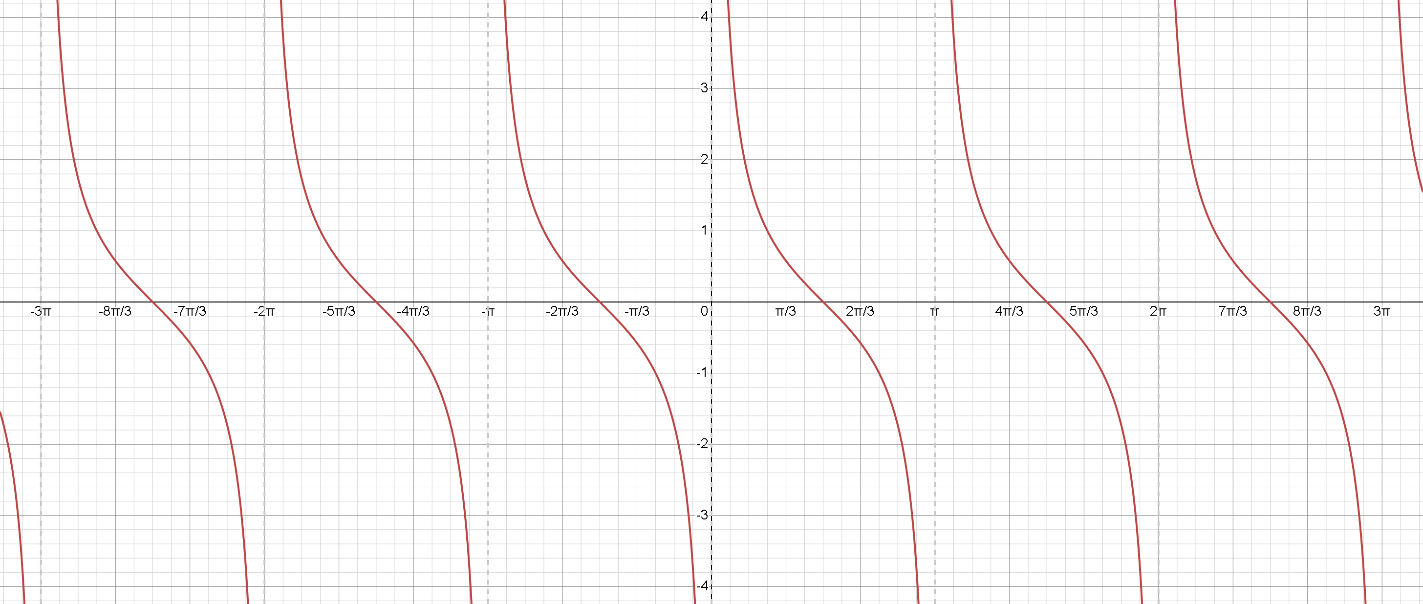
2. Cotangent Function cot(x):
The cotangent function is defined as the ratio of the cosine function to the sine function, i.e.
\( cot(x) = \frac{cos(x)}{sin(x)} \)

Key features of the cotangent graph:

• Period: The cotangent function has a period of \( \pi \), which means it repeats itself every \( \pi \) units along the \(x\)-axis, just like the tangent function.
• Asymptotes: Since the cotangent function is the ratio of cosine and sine, it is undefined when the sine function equals zero. This occurs at integer multiples of \(\pi\). (0, \( \pm \pi\), \( \pm 2 \pi \), and so on). These points are where the vertical asymptotes occur.
• Range: The range of the cotangent function is \( (- \infty, \infty ) \), as the function takes on all real values.
• Symmetry: The cotangent function is an odd function, which means it is symmetric with respect to the origin.
  In other words, \(cot(-x)=-cot(x)\).
• Decreasing: The cotangent function is always decreasing over each of its periods.

In summary, both tangent and cotangent functions are periodic, with a period of \( \pi \), and exhibit odd symmetry. They have different vertical asymptotes and behavior, with the tangent function being increasing while the cotangent function is decreasing.

Inverse trigonometric functions ☰

Inverse trigonometric functions, also known as arc-functions or anti-trigonometric functions, are the inverse functions of the basic trigonometric functions: sine, cosine, and tangent. These functions allow you to find the angle when you know the trigonometric value. There are six main inverse trigonometric functions:

1. Inverse Sine. \( sin^{-1} (x) \) or \( arcsin(x) \):
The inverse of the sine function.
Domain: \( [-1 , 1 ] \)
Range: \( [- \frac{ \pi }{2}, \frac{ \pi }{2} ] \)

2. Inverse Cosine. \( cos^{-1} (x) \) or \( arccos(x) \):
The inverse of the cosine function.
Domain: \( [-1 , 1 ] \)
Range: \( [ 0 , \pi ] \)

3. Inverse Tangent. \( tan^{-1} (x) \) or \( arctan(x) \):
The inverse of the tangent function.
Domain: ( \(- \infty , \infty \) )
Range: ( \( - \frac{ \pi }{2}, \frac{ \pi }{2} \) )

4. Inverse Cosecant. \( csc^{-1} (x) \) or \( arccsc(x) \):
The inverse of the cosecant function (which is the reciprocal of the sine function).
Domain: \( (-\infty, -1] \cup [1, \infty) \)
Range: \( \left[-\frac{\pi}{2}, 0\right) \cup \left(0, \frac{\pi}{2}\right]\)

5. Inverse Secant. \( sec^{-1} (x) \) or \( arcsec(x) \):
The inverse of the secant function (which is the reciprocal of the cosine function).
Domain: \( \left(-\infty, -1\right] \cup \left[1, \infty\right) \)
Range: \( \left[0, \frac{\pi}{2}\right) \cup \left(\frac{\pi}{2}, \pi\right] \)

6. Inverse Cotangent. \( cot^{-1} (x) \) or \( arccot(x) \):
The inverse of the cotangent function.
Domain: ( \(- \infty , \infty \) )
Range: ( \( 0 , \pi \) )


Properties of inverse trigonometric functions:

⠐ Restricted domains and ranges: To make trigonometric functions invertible, their domains are restricted, which results in restricted ranges for the inverse trigonometric functions.

⠐ Notation: Inverse trigonometric functions are often denoted with a "\( ^{-1} \)" or " \(arc\)" prefix. For example, \( sin^{-1} (x) \) or \(arcsin(x) \) represent the inverse sine function.
Note that \( sin^{-1} (x) \) is NOT the same as \( \frac{1}{sin(x)} \) , which is the reciprocal function (cosecant).

⠐ Composition:
The composition of a trigonometric function and its inverse function results in the identity function, provided that the input is within the correct range:

\( sin( arcsin(x) ) = x \), If \(x\) is in the domain of \( arcsin( [-1,1] ) \)

\( arcsin ( sin(x) ) = x \), If \(x\) is in the range of \( arcsin( [ -\frac{ \pi }{2} , \frac{ \pi }{2} ] ) \)

Similar relationships hold for the other inverse trigonometric functions.

⠐ Differentiability:
Inverse trigonometric functions are differentiable within their domains, except at points where the original trigonometric functions have vertical tangents.
For example, the inverse sine and cosine functions are not differentiable at \(x=-1\) and \(x=1\), and the inverse tangent function is not differentiable at \(x=- \infty \) and \(x= \infty \).

⠐ Symmetry:
Some inverse trigonometric functions exhibit symmetry.
For example:
\( arctan(-x) = -arctan(x) \) : The inverse tangent function is an odd function.

\( arccot(-x) = \pi - arcctg(x) \) : The inverse cotangent function exhibits a specific type of symmetry.

Inverse trigonometric functions are crucial for solving problems involving triangles and trigonometry, especially when you need to find an angle given the lengths of the sides or other trigonometric values. They are used in various fields of mathematics, physics, and engineering, such as in calculus, geometry, and the study of periodic phenomena.

⠐ Derivatives:
The derivatives of the inverse trigonometric functions are essential in calculus, particularly when solving integration problems involving trigonometric functions. Here are the derivatives of the three primary inverse trigonometric functions:

\( \frac{d (\arcsin(x))}{dx} = \frac{1}{\sqrt{1 - x^2}} \)

\( \frac{d (\arccos(x))}{dx} = -\frac{1}{\sqrt{1 - x^2}} \)

\( \frac{d (\arctan(x))}{dx} = \frac{1}{1 + x^2} \)