Polynomial equation of degree (Higher-degree polynomial equations)
A polynomial equation of degree is an equation of the form where are constants and is a non-negative integer. Here, is the variable.
The degree of a polynomial equation is the highest power of the variable x in the equation.
For example, the equation is a polynomial equation of degree 3, because the highest power of is 3. The constant term is also included in the sum, even though it does not involve , to make it clear that this is a polynomial equation.
The solutions of a polynomial equation of degree are called roots or zeros of the polynomial. The Fundamental Theorem of Algebra states that a polynomial of degree has exactly complex roots, counting multiplicities. This means that there are exactly solutions to the equation , when we allow
complex values of .
There are several techniques for finding the roots of polynomial equations of degree . For example, if , then the equation has a single root, which is . For quadratic equations of the form , we can use the quadratic formula to find the roots. For cubic equations of the form , there is
also a formula called
Cardano's formula
, which gives the roots in terms of the coefficients , , , . However, this formula can be quite complicated to use in practice. For polynomial equations of degree greater than 3, there is no general formula that gives the roots in terms of the coefficients, although there are some special cases where the roots can be found using other methods.
In general, finding the roots of a polynomial equation of degree n involves factoring the polynomial into linear and quadratic factors, and then solving each of the factors separately.
For example, consider the polynomial equation . We can factor this as , which gives us three solutions: , and . These are the roots of the polynomial equation.
Higher-degree polynomial equations
are equations of degree 4 or higher, such as quartic equations and quintic equations . These equations can be more difficult to solve than lower-degree polynomial equations and may require more advanced techniques, such as the use of complex numbers and group theory.
One important result in the theory of polynomial equations is the fundamental theorem of algebra, which states that every non-constant polynomial equation with complex coefficients has at least one complex root. This means that even if a polynomial equation cannot be solved using real numbers, it can always be solved using complex numbers.
There are several techniques for solving higher-degree polynomial equations. One approach is to try to factor the equation into simpler polynomials.
For example, the quartic equation can be factored as , which has roots and . However, not all higher-degree polynomial equations can be factored in this way.
Another approach is to use numerical methods to approximate the roots of the equation. For example, the Newton-Raphson method can be used to iteratively find better and better approximations to the roots. However, these methods do not guarantee an exact solution and may require a large number of iterations to converge.
For quintic and higher-degree polynomial equations, there is no general formula for finding the roots in terms of the coefficients, as there are for quadratic, cubic, and quartic equations. This was proved by the mathematician Évariste Galois in the 19th century, using the theory of group theory. Instead, specific equations can be solved using specialized techniques
or approximated using numerical methods.
Rational equations
Rational equations are equations that involve rational expressions, which are ratios of two polynomials. A polynomial is an expression that consists of one or more terms involving variables with whole-number exponents and coefficients that can be real numbers or complex numbers.
Rational equations are typically written in the form: , where , , and are polynomials, and and .
The main goal when solving rational equations is to find the values of the variable that make the equation true. To solve a rational equation, the first step is to clear denominators by multiplying both sides of the equation by a common denominator of the two rational expressions. This can be found by multiplying the denominators and and
simplifying the resulting expression. After clearing denominators, the equation becomes a polynomial equation, which can be solved using standard algebraic techniques. Once the solutions for x are found, it is important to check them in the original equation to ensure they are valid solutions. If a solution makes one or both denominators equal to zero, it is not a
valid solution and must be excluded.
Example: Solve the equation .
Step 1: Find a common denominator. In this case, the common denominator is , so we can rewrite the equation as:
;
Simplifying, we get:
;
Combining the fractions, we get:
Step 2: Eliminate the denominators by multiplying both sides of the equation by the common denominator: .
Step 3: Solve for . .
Step 4: Check for extraneous solutions. Since makes the denominator non-zero, there are no extraneous solutions to check.
Therefore, the solution to the equation is .
Absolute value equation
An absolute value equation is a type of equation that involves the absolute value of a variable. The absolute value of a number is the distance from zero on the number line, so the absolute value of a variable can be thought of as the distance from zero that the variable can take.
The general form of an absolute value equation is: , where is some expression that contains the variable and is another expression that may or may not contain . The goal in solving an absolute value equation is to find all values of that make the equation true. The basic approach to solving absolute value equations
is to split the equation into two cases, one where is positive and another where is negative. This is because the absolute value of a positive number is the number itself, while the absolute value of a negative number is its opposite. So, if we know whether is positive or negative, we can determine the value of and solve the
equation.
For example, consider the equation: .
We start by splitting this into two cases:
Case 1: is positive.
.
.
Case 2: is negative.
.
.
.
Therefore, the solutions to the equation are and .
It is also possible for an absolute value equation to have no solutions. For example, consider the equation: .
Since the absolute value of any number is always non-negative, there is no value of that makes the left side of the equation equal to a negative number. Therefore, this equation has no solutions.
In summary, solving absolute value equations involves splitting the equation into two cases based on whether the expression inside the absolute value is positive or negative, solving each case separately, and then combining the solutions. It is important to check that any solutions we find actually satisfy the original equation, as some equations may have no
solutions or extraneous solutions that do not actually work.
Irrational equations
Irrational equations are equations that involve one or more irrational functions or irrational expressions. An irrational function is a function that cannot be expressed as a ratio of two polynomials. Common examples of irrational functions include the square root function , the cube root function and the logarithmic
function .
The general form of an irrational equation is: , where and are both irrational functions or expressions. Solving such equations usually involves isolating the irrational expression on one side of the equation and then squaring both sides, which can eliminate the radical. However, this method can introduce extraneous solutions, which
are solutions that do not satisfy the original equation.
To illustrate this, consider the following example: .
To solve this equation, we can square both sides:
However, we must check our solution to make sure it is not extraneous.
Equations in two variables. System of equations.
Equations in two variables are mathematical expressions that relate two variables, typically denoted by and , with an equality sign. These types of equations are represented in the form: , where , , are constants, and are variables. The values of and that satisfy the equation are called solutions or
roots of the equation.
The graph of an equation in two variables is a straight line in the Cartesian coordinate plane, where is the horizontal axis and is the vertical axis. The slope-intercept form of the equation of a line is: , where is the slope of the line and is the -intercept, which is the point where the line crosses the -axis.
To convert an equation in the standard form to the slope-intercept form, we can solve for :
Thus, the slope of the line is and the -intercept is .
Conversely, to convert an equation in the slope-intercept form to the standard form, we can rearrange the terms:
where and and .
To solve a system of two equations in two variables, we need to find the values of and that satisfy both equations simultaneously. One way to do this is by graphing the two equations and finding the point where the lines intersect. This point represents the solution of the system.
Another method to solve a system of two equations in two variables is by substitution. In this method, we solve one of the equations for one of the variables and substitute the expression into the other equation. This will result in an equation in one variable, which we can solve to find the value of the variable. We can then substitute this value back into one of
the original equations to find the value of the other variable.
For example, consider the system of equations:
Solving the second equation for , we get: .
Substituting this expression into the first equation, we get: .
Simplifying and solving for , we get: , .
Substituting this value back into the equation , we get: , .
Therefore, the solution of the system is .
In summary, equations in two variables are mathematical expressions that relate two variables with an equality sign, and their graphs are straight lines in the Cartesian coordinate plane. To solve a system of two equations in two variables, we can use graphing or substitution methods to find the values of and that satisfy both equations simultaneously.
System of equations.
A system of equations is a set of two or more equations with the same variables. The variables in a system of equations represent the same values in each equation. We can solve a system of equations by finding the values of the variables that satisfy all of the equations in the system.
There are different methods to solve a system of equations, such as graphing, substitution, and elimination. The method we choose depends on the complexity of the system and personal preference.
One way to solve a system of equations is by graphing. Graphing allows us to visualize the solutions of the system as the intersection points of the graphs of the equations. To graph the equations, we plot points on the Cartesian plane that satisfy each equation, then connect the points to form lines. The intersection points of the lines represent the solutions of
the system.
For example, consider the system of equations:
Example: let's solve the following system of equations by graphical method.
To graph these equations, we can choose several values of and plug them into each equation to find the corresponding values of . Then we plot the resulting points and connect them to form the lines.
For the first equation:
| -2 | -3 |
| -1 | -1 |
| 0 | 1 |
| 1 | 3 |
| 2 | 5 |
For the second equation:
| -3 | 5 |
| 0 | 4 |
| 3 | 3 |
We can now plot these points and connect them to form the lines:
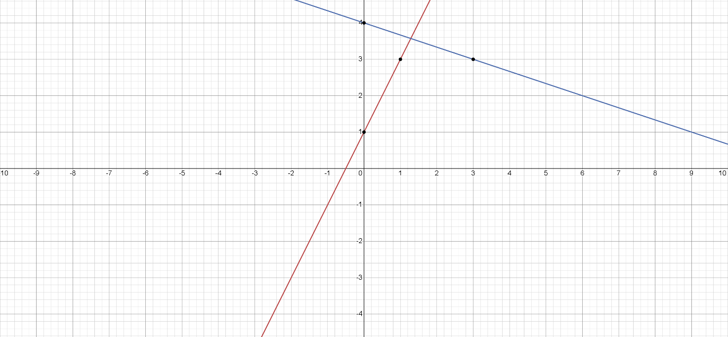
The intersection point of the lines is the solution of the system, which is approximately .
Another method to solve a system of equations is by substitution. In this method, we solve one of the equations for one of the variables, then substitute the expression into the other equation. This results in an equation in one variable, which we can solve to find the value of the variable. We can then substitute this value back into one of the original equations
to find the value of the other variable.
System of equations in which one equation is first-degree and the other equation is second-degree
A system of equations is a set of equations that are considered together as a group. A system of equations in which one equation is first-degree (linear) and the other equation is second-degree (quadratic) is a type of non-linear system of equations.
The general form of a first-degree equation is , where and are constants and is the variable.
The general form of a second-degree equation is , where , and are constants and is the variable.
To solve a system of equations in which one equation is first-degree and the other equation is second-degree, there are several methods, including:
- Substitution Method: In this method, we solve one of the equations for one of the variables in terms of the other variable, and then substitute this expression into the other equation. This results in a quadratic equation in one variable, which we can solve using the quadratic formula or factoring. Once we have found the value(s) of the variable, we can substitute back into one of the original equations to find the value(s) of the other variable.
- Elimination Method: In this method, we eliminate one of the variables by multiplying one or both equations by a constant, such that the coefficients of one of the variables are equal and opposite in the two equations. This results in an equation in one variable, which we can solve and then substitute back into one of the original equations to find the value(s) of the other variable.
For example, consider the following system of equations:
From the second equation, we can factor out a common factor of as .
This gives us two possibilities: or
If we solve the first equation for as , we can substitute this into the second equation to get:
This simplifies to , which is true for any value of . Therefore, we have infinitely many solutions, which can be expressed as , where is any real number.
If we solve the second equation for as , we can substitute this into the first equation to get:
Substituting this into , we get . Therefore, we have one solution, which is .
Graphical Method:
In this method, we graph both equations on the same coordinate plane and look for the point(s) of intersection, which represent the solutions to the system of equations. However, this method may not always be feasible for complex systems of equations.
In conclusion, a system of equations in which one equation is first-degree and the other equation is second-degree can be solved using various methods, including substitution, elimination, and graphical methods. The choice of method depends on the specific system of equations and the individual preferences of the solver.
System of two second-degree equations in two variables
A system of two second-degree equations in two variables is a set of two equations in two variables where each equation is a second-degree polynomial. The general form of such a system is:
where , , , , , , , , , are constants and , are the variables.
This type of system is nonlinear, which means that the solutions to the system do not necessarily form a straight line. Instead, the solutions may be curves or sets of discrete points in the -plane.
To solve this system, one possible method is to use substitution to eliminate one variable and reduce the system to a single equation in one variable. This involves solving one of the equations for either x or y, and then substituting that expression into the other equation. The resulting equation will be a single second-degree polynomial in one variable, which can
be solved using techniques such as factoring or the quadratic formula.
Another possible method is to use the method of elimination, which involves adding or subtracting the two equations to eliminate one of the variables. This can be done by multiplying one or both equations by constants, as needed, to create coefficients that will cancel out when the equations are added or subtracted.
The solutions to the system will be the values of and that satisfy both equations simultaneously. Depending on the specific equations in the system, there may be one or more solutions, or no solutions at all. Graphing the equations in the xy-plane can provide a visual representation of the possible solutions, and can help in understanding the behavior of
the system.
An example of a system of two second-degree equations in two variables is:
This system represents the intersection of a circle centered at the origin with radius 5, and a hyperbola with vertical axis and centered at the origin.
" src="imageforhtm/s9-5-2.webp" loading="lazy" />
With this graph, we can say that the system has four solutions.
Adding the two equations, we obtain:
.
Taking the square root of both sides, we get . Substituting these values back into one of the original equations, we can solve for . For example, using the first equation, we have:
Therefore, the solutions to the system are:
,
,
.